.comment-link {margin-left:.6em;}

Oracle Sponge -- Now Moved To Wordpress

Please use http://oraclesponge.wordpress.com

Tuesday, December 27, 2005

"The Economist" Premium Content Free

OK, you have to watch a short commercial, but that's capitalism folks. And it's a small price of entry for the world's best world affairs and business coverage.

http://www.economist.com

Tuesday, December 20, 2005

The Tranquility of Materialized Views

Yesterday evening I searched the Oracle 10g documentation for the string "materialized views", and was browsing through the 378 matching entries in "Error Messages". At about the point where I got to ORA-12055: materialized view definition contains cyclic dependencies with existing materialized views I was overcome with a great sense of tranquility and understanding of materialized views.

Shortly after that I realised that I was probably delusional from lack of sleep or something, so I snapped out of it and went to bed. Is it still only Tuesday today?

Saturday, December 17, 2005

Optimizing Materialized Views Part V: HOLAP Query Performance

HOLAP Performance With Different Aggregation Levels

I'm going to construct a slightly different test data set for this experiment, involving the aggregation of 10,000,000 by three different columns each having around 1000 distinct values.

drop table master;

create table master
(
col1 not null,
col2 not null,
col3 not null,
tx_qty not null
)
pctfree 0
nologging
as
select
trunc(dbms_random.value(1,1000)),
trunc(dbms_random.value(1,100),2)
from
dual
connect by
1=1 and
level <= 1000000;

The performance test queries will take the form of a query such as the following:

clear screen
alter session set workarea_size_policy = manual;
alter session set sort_area_size = 1000000000;
alter session set sort_area_retained_size = 1000000;
set timing on autotrace on feedback off

-- loop: the following executed four times
alter system flush buffer_cache;
select sum(s_tx_qty) from
(Select
sum(tx_qty) s_tx_qty,
{grouped column list}
From master group by grouping sets
({grouping sets});
-- end of loop

In the four executions of the query the first invokes a hard parse and the autotrace statistics are discarded. The autotrace results of the following three results are averaged.

We will try aggregations at a number of different levels. Some of these will involve hierarchies and some will not, but the aim is to expose as full a range of optimizations as we can. For the sake of my time, my sanity, and blog length I'm going to run these to get simple wall clock times and autotrace statistics for now. The host machine and database will be as quiescent as possible.

We'll start with simple, conventional aggregations to get benchmarks for familiar operations.


Benchmark 1

Benchmark 2

Benchmark 3

Benchmark 4

Group By

None

col1

col1,col2

Col, col2, col3

rows

1

999

997,955

9,949,574

consistent gets

25,074

25,074

25,074

25,074

physical reads

25,062

25,062

25,062

25,062

sorts (memory)

0

1

1

1

Elapsed Time

8.87

18.95

59.70

92.42


In the following table we present the results of the various grouping set tests, with the “Y” indicating that the grouping set was included as part of that test.

Grouping Set(s) Used

Test 1

Test 2

Test 3

Test 4

Test 5

Test 6

Test 7

Test 8

()

Y


Y

Y

Y

Y

Y

Y

(COL1)


Y

Y

Y

Y

Y

Y

Y

(COL2)


Y

Y

Y


Y

(COL3)


Y


Y

(COL1,COL2)


Y

Y

Y

Y

(COL1,COL3)


Y


Y

(COL2,COL3)


Y


Y

(COL1,COL2,COL3)


Y

Y

rows

1

999

1,000

1,999

999,954

2,996,849

10,948,529

12,946,423

recursive calls

0

0

0

185

25

299

270

319

db block gets

0

0

0

23,575

2803

38,219

34745

40,872

consistent gets

25,074

25,074

25074

71,498

33286

122,911

62313

130,765

physical reads

25,062

25,062

25062

71,434

27799

122,776

62242

130,622

redo size

0

0

0

1,929

2,147

3525.33

1513

3,080

sorts (memory)

0

1

1

2

3

4

2

4

sorts (disk)

0

0

0

0

0

0

0

0

Elapsed Time

12.33

16.34

17.84

63.57

71.49

230.23

173.08

266.69


Test 1 is a straight aggregation to find the sum of tx_qty, but expressed as a grouping set of () rather than the usual “Select Sum(my_col) From my_table” syntax. The autotrace statistics are also very conventional and show physical reads very close to consistent gets, with no db block gets or recursive SQL.

This test is logically the same as Benchmark 1, but required an elapsed time 50% longer. The execution plans are in fact different, with the SORT AGGREGATE of the conventional method being replaced with a SORT GROUP BY NOSORT in the grouping sets method.

Test 2 is similarly conventional, finding the sum of tx_qty grouped by col1. Again this is expressed as a grouping set (col1) rather than the regular syntax and the autotrace statistics are very similar to Test 1 with the addition of an in-memory sort. The performance is very similar to that of Benchmark 2, to which it is logically equivalent, and both queries are using a SORT GROUP BY operation.

Test 3 gives our first hierarchical result set, combining the results of Test 1 and Test 2. In fact the result set for Test 3 is logically equivalent to (Benchmark1 UNION ALL Benchmark 2), and the benefits of the HOLAP cube begin to show themselves. The average elapsed time of 17.84 seconds is only 62% of the elapsed times for Tests 1 and 2 combined. The execution plan shows a SORT (GROUP BY ROLLUP) operation which is evidently an optimization specifically for hierarchical cube queries. It appears either that the result for the (COL1) grouping set is being used as the basis for the () grouping set calculation, or that the results for both sets are being computed in the same operation. As we will shortly see, the latter appears to be the more probable scenario.

Test 4 adds into Test 3 a grouping set of (Col2), giving two sets at the same level with no more detailed level included. This result ought to be logically similar to (Test 2 UNION ALL Test 3) -- with the appropriate columns being used -- or (Benchmark 1 UNION ALL Benchmark 2 UNION ALL Benchmark 3). The result is surprising because this time the performance is well in excess of those comparisons, and gives the first hint at a possible contra-indication for HOLAP cube MV's. The elapsed time of 63.57 seconds is 86% higher than the sum of the elapsed times for Tests 2 and 3, of 34.18 seconds.

The explain plan show the creation of two temporary tables, although when the statement is executed these temporary table names are of course different.

------------------------------------------------------------------------------------------------------------
| Id | Operation | Name | Rows | Bytes | Cost (%CPU)| Time |
------------------------------------------------------------------------------------------------------------
| 0 | SELECT STATEMENT | | 1 | | 170 (85)| 00:00:02 |
| 1 | SORT AGGREGATE | | 1 | | | |
| 2 | VIEW | | 707K| | 170 (85)| 00:00:02 |
| 3 | TEMP TABLE TRANSFORMATION | | | | | |
| 4 | LOAD AS SELECT | | | | | |
| 5 | TABLE ACCESS FULL | MASTER | 10M| 114M| 162 (88)| 00:00:02 |
| 6 | LOAD AS SELECT | | | | | |
| 7 | SORT GROUP BY | | 1 | 26 | 3 (34)| 00:00:01 |
| 8 | TABLE ACCESS FULL | SYS_TEMP_0FD9D6665_1214756C | 1 | 26 | 2 (0)| 00:00:01 |
| 9 | LOAD AS SELECT | | | | | |
| 10 | SORT GROUP BY ROLLUP | | 1 | 26 | 3 (34)| 00:00:01 |
| 11 | TABLE ACCESS FULL | SYS_TEMP_0FD9D6665_1214756C | 1 | 26 | 2 (0)| 00:00:01 |
| 12 | VIEW | | 1 | 39 | 2 (0)| 00:00:01 |
| 13 | TABLE ACCESS FULL | SYS_TEMP_0FD9D6666_1214756C | 1 | 39 | 2 (0)| 00:00:01 | ------------------------------------------------------------------------------------------------------------

Here are the STAT lines from a 10046 trace file:

STAT #6 id=1 cnt=1999 pid=0 pos=1 obj=0 op='TEMP TABLE TRANSFORMATION  (cr=71632 pr=66687 pw=23191 time=58587487 us)'
STAT #6 id=10 cnt=1999 pid=1 pos=1 obj=0 op='VIEW (cr=144 pr=6 pw=0 time=27785 us)'
STAT #6 id=11 cnt=1999 pid=10 pos=1 obj=-40016278 op='TABLE ACCESS FULL SYS_TEMP_4254951018 (cr=144 pr=6 pw=0 time=19771 us)'
STAT #6 id=12 cnt=1 pid=1 pos=2 obj=0 op='LOAD AS SELECT (cr=25074 pr=20328 pw=23185 time=19896368 us)'
STAT #6 id=13 cnt=10000000 pid=2 pos=1 obj=260950 op='TABLE ACCESS FULL OBJ#(260950) (cr=25074 pr=20328 pw=0 time=30000104 us)'
STAT #6 id=14 cnt=1 pid=1 pos=3 obj=0 op='LOAD AS SELECT (cr=23208 pr=23185 pw=3 time=18510637 us)'
STAT #6 id=15 cnt=999 pid=4 pos=1 obj=0 op='SORT GROUP BY (cr=23208 pr=23185 pw=0 time=18508219 us)'
STAT #6 id=16 cnt=10000000 pid=5 pos=1 obj=-40016279 op='TABLE ACCESS FULL SYS_TEMP_4254951017 (cr=23208 pr=23185 pw=0 time=30022328 us)'
STAT #6 id=17 cnt=1 pid=1 pos=4 obj=0 op='LOAD AS SELECT (cr=23206 pr=23168 pw=3 time=20142290 us)'
STAT #6 id=18 cnt=1000 pid=7 pos=1 obj=0 op='SORT GROUP BY ROLLUP (cr=23206 pr=23168 pw=0 time=20140880 us)'
STAT #6 id=19 cnt=10000000 pid=8 pos=1 obj=-40016279 op='TABLE ACCESS FULL SYS_TEMP_4254951017 (cr=23206 pr=23168 pw=0 time=30018947 us)'

Cleaned up a little, this reads more easily as:

TEMP TABLE TRANSFORMATION
VIEW
TABLE ACCESS FULL SYS_TEMP_4254951018
LOAD AS SELECT
TABLE ACCESS FULL OBJ#(260950)
LOAD AS SELECT
SORT GROUP BY
TABLE ACCESS FULL SYS_TEMP_4254951017
LOAD AS SELECT
SORT GROUP BY ROLLUP
TABLE ACCESS FULL SYS_TEMP_4254951017

The temporary table definitions are as follows:

CREATE GLOBAL TEMPORARY TABLE "SYS"."SYS_TEMP_0FD9D6669_1214756C"
("C0" NUMBER,
"C1" NUMBER,
"A0" NUMBER )
IN_MEMORY_METADATA CURSOR_SPECIFIC_SEGMENT STORAGE (OBJNO 4254951017 ) NOPARALLEL;

CREATE GLOBAL TEMPORARY TABLE "SYS"."SYS_TEMP_0FD9D666A_1214756C"
("C0" NUMBER,
"C1" NUMBER,
"D0" NUMBER,
"A0" NUMBER )
IN_MEMORY_METADATA CURSOR_SPECIFIC_SEGMENT STORAGE (OBJNO 4254951018 ) NOPARALLEL

You'll note that the global temporary tables' OBJNO clause correlate to part of the temporary table name referenced in the STAT lines – a bit unintuitive that, if you ask me.

So how do we interpret this? Fortunately, a 10046 trace file contains some interesting clues.

Although it shows the creation of the temporary tables it does not reveal any other recursive SQL against them. However it does show wait events of course, and where there is a 'db file scattered read' there are also p1 and p2 parameters which tell you the file number and block number respectively for the object being read. Now the only objects involved here ought to be our MASTER table and our two temporary tables, and we know the file and block numbers for the MASTER table are available from DBA_EXTENTS.

So I'm going to break off there for this entry, and present the analysis of the execution plan, and more, next time.

Thursday, December 15, 2005

An International Community, Apparantly

I recently increased my StatCounter log size to 1,000 -- more from boredom than any real need, admittedly -- and have found it fascinating to see the range of countries that the Sponge gets visits from. Here is my current list:


Country Visits
=============== ======
United States: 209
United Kingdom: 72
Australia: 26
Switzerland: 21
Canada: 20
Sweden: 12
Unknown: 12
India: 11
Greece: 9
Germany: 9
Netherlands: 6
Turkey: 6
Luxembourg: 5
Singapore: 5
Slovenia: 4
France: 4
Denmark: 4
Spain: 4
Estonia: 3
Hong Kong: 2
Romania: 2
Belgium: 2
Ukraine: 2
Serbia And Montenegro: 1
Saudi Arabia: 1
Egypt: 1
Lebanon: 1
Japan: 1
Czech Republic: 1
Lithuania: 1
Austria: 1
Finland 1


As you see, Septics lead the way, followed closely by other English speaking countries.

Being the well-travelled International Citizen that I am, I'm a little embarrassed that I sometimes get goggly at the thought of all these far-away places, and also that I use non-words like "goggly" and "septic" to an international audience. I catch myself thinking dumb things like, "Wow! They have databases in Lithuania!?!?". Yes dumbass, they also have cars and washing machines as well, I expect.

Anyway, a question: what do people use for support in the smaller countries of the world? Do Oracle have national support staff speaking the local language(s), or do you rely on a regional system where the major regional languages are spoken, or do you have to fall back on knowledge of English and contact Oracle's global support people? I was trying to find out a while back whether Oracle published their documentation in any languages other than English, but pretty much drew a blank on it.

Tuesday, December 13, 2005

Reunited With Old Technology

While standing on a chair in my basement storage room to make tweaks to my Shelf Of Technology, I was distracted by an aluminium case that I'd been carrying from abode to abode for about fifteen years without opening it as far as I could recall. Nestled snugly inside the blue foam padding within was my first proper camera, a Pentax ME Super.

It's been a while since I've handled it, and it felt heavy, solid, and just a delight to hold. After fifteen years, did it still work?

Away to a local store for a pair of LR44 batteries and the smallest roll of film available. Straightaway more memories came back. The batteries go in "+" side down, and they always try and flip themselves over. The little white button that has to be pressed to change the shutter action is fiddly. Little LEDs in the view finder tell you the shutter speed it will choose on the Auto setting. And it still feels heavy, especially after a few years with my Sony Cybershot digital.

The first roll of file flew by. It was really too dark for an ISO100 so I had to find kids at their most stationary, which any parent can tell you means that they were just sitting mostly still but vibrating slightly with surplus energy -- on average, they were not moving. The light was artificial so it had a warm cast to it that the flash on the digital camera would have obscured.

So here's the results so far.


The photo CD does not give great resolution and the 35mm aspect ratio is a little different, but so far it's encouraging enough for an investment in three rolls of faster black and white film. Some of the reviews I've read of this model mention its strength with black and white in particular, so now I need a chance to get up into the mountains to try it out so my creative urges have outlets other than endless images of the cat, the kids and the strata of detritus on my desk.

Playing With System Statistics

Updated 14-Dec-2005 at the end of the article

I was just musing on what we can deduce directly from system statistics, and thought of the following.

If the system recorded the average MBRC and the average MREADTIM over the period of statistics collection, then does that mean that we can learn something directly about the performance of the i/o system during that time? I ran an experiment:

drop table t
/

create table t
nologging
pctfree 99
pctused 0
tablespace REG_UA4MB_MSSM
as
select rpad(rownum,100) whatever
from dual
connect by 1=1 and
level < estimate_percent=""> 1,block_sample => true)

select blocks*
(select block_size
from user_tablespaces
where tablespace_name = 'REG_UA4MB_MSSM')
/1024/1024 table_size_Mb
from user_tables
where table_name = 'T'
/

alter system flush buffer_cache;

exec dbms_stats.gather_system_stats('START')

select count(*) from t;

exec dbms_stats.gather_system_stats('STOP')

select pname,
pval1
from sys.aux_stats$
where sname = 'SYSSTATS_MAIN'
/

select (select pval1
from sys.aux_stats$
where sname = 'SYSSTATS_MAIN' and
pname = 'MBRC') *
(select to_number(value) block_size
from v$parameter
where name = 'db_block_size') /
(select pval1
from sys.aux_stats$
where sname = 'SYSSTATS_MAIN' and
pname = 'MREADTIM')
/1024 sys_stat_mread_speed
from dual
/


What I'm doing there is creating a table of around 512Mb (because I'm aiming for one row per block, and each block is 8kb), flushing the buffer cache, starting the collection of system statistics, timing a select of count(*) for the 512Mb table, and comparing the read speed according to table_size/duration against MBRC*block_size/MREADTIM.

In fact the correlation is pretty good. Here's my own execution of the above script with timing on:


SQL> drop table t
2 /

Table dropped.

Elapsed: 00:00:00.37
SQL>
SQL> create table t
2 nologging
3 pctfree 99
4 pctused 0
5 tablespace REG_UA4MB_MSSM
6 as
7 select rpad(rownum,100) whatever
8 from dual
9 connect by 1=1 and
10 level <>
SQL> exec dbms_stats.gather_table_stats(user,'T',estimate_percent=> 1,block_samp
le => true)

PL/SQL procedure successfully completed.

Elapsed: 00:00:04.29
SQL>
SQL> select blocks*
2 (select block_size
3 from user_tablespaces
4 where tablespace_name = 'REG_UA4MB_MSSM')
5 /1024/1024 table_size_Mb
6 from user_tables
7 where table_name = 'T'
8 /

TABLE_SIZE_MB
-------------
511.992188

Elapsed: 00:00:00.06
SQL>
SQL> alter system flush buffer_cache;

System altered.

Elapsed: 00:00:00.01
SQL>
SQL> exec dbms_stats.gather_system_stats('START')

PL/SQL procedure successfully completed.

Elapsed: 00:00:00.28
SQL>
SQL> select count(*) from t;

COUNT(*)
----------
65535

Elapsed: 00:00:13.12
SQL>
SQL> exec dbms_stats.gather_system_stats('STOP')

PL/SQL procedure successfully completed.

Elapsed: 00:00:00.04
SQL>
SQL> select pname,
2 pval1
3 from sys.aux_stats$
4 where sname = 'SYSSTATS_MAIN'
5 /

PNAME PVAL1
------------------------------ ----------
CPUSPEEDNW 1132.397
IOSEEKTIM 10
IOTFRSPEED 4096
SREADTIM 11.039
MREADTIM 11.886
CPUSPEED 1084
MBRC 63
MAXTHR 36093952
SLAVETHR 2065408

9 rows selected.

Elapsed: 00:00:00.00
SQL>
SQL> select (select pval1
2 from sys.aux_stats$
3 where sname = 'SYSSTATS_MAIN' and
4 pname = 'MBRC') *
5 (select to_number(value) block_size
6 from v$parameter
7 where name = 'db_block_size') /
8 (select pval1
9 from sys.aux_stats$
10 where sname = 'SYSSTATS_MAIN' and
11 pname = 'MREADTIM')
12 /1024 sys_stat_mread_speed
13 from dual
14 /

SYS_STAT_MREAD_SPEED
--------------------
42.4028269

Elapsed: 00:00:00.00


So the system statistics suggest a multiblock read performance of 42.4Mb/sec, and the Count(*) timing of 13.12sec and table size of 512Mb suggest 39Mb/sec.

This is just a single-threaded multiblock read on an otherwise quiescent system and so probably represents the upper limit on what this system could achieve, rather than what it would achieve in a multiuser environment, but the method seems useful as some kind of benchmark. Shouldn't it be possible to perform some kind of real-world comparison on this basis, if the system stats were collected during a period of multiuser activity?

I intuitively feel that this calculation would represent an approximation of how many Mb/sec you could expect from each thread of a parallel query, providing that neither the CPUs nor the disk subsystem are choking performance. So if you knew that you could run a degree 8 scan of a table without any part of the system choking, this ought to tell you hw long such a scan would take.

I think.

Update 14-Dec-2005

Following comments by Jonathan Lewis I ran a slightly modified version of the script to start a 10046 level 8 trace before the start of system statistics gathering. Here's a summary in which I've just included truncated SQL statements and wait events (and summarized those where appropriate):


BEGIN dbms_stats.gather_system_stats('START'); END;
SELECT /*+ rule */ VALUE FROM V$PARAMETER WHERE UPPER(NAME) = 'STATISTICS_LEVEL'
SELECT S.SNAME, S.PNAME, S.PVAL1, S.PVAL2 FROM AUX_STATS$ S WHERE S.SNAME LIKE 'S
WAIT #2: nam='db file sequential read' ela= 230 p1=1 p2=4434 p3=1
WAIT #2: nam='db file sequential read' ela= 139 p1=1 p2=4426 p3=1
SELECT SUM(KCFIOSBR) SBLKRDS, SUM(KCFIOSBT)*10 SBLKRDTIM, SUM(KCFIOMBR) MBLKRDS,
SELECT S1.VALUE - S2.VALUE MBREADS FROM V$SYSSTAT S1, V$SYSSTAT S2 WHERE S1.NAME
delete from sys.cache_stats_0$
WAIT #20: nam='db file sequential read' ela= 8581 p1=1 p2=5425 p3=1
WAIT #20: nam='db file scattered read' ela= 1069 p1=1 p2=5426 p3=7
WAIT #20: nam='db file scattered read' ela= 10004 p1=1 p2=51393 p3=8
WAIT #20: nam='db file scattered read' ela= 13039 p1=1 p2=64049 p3=8
WAIT #20: nam='db file scattered read' ela= 3618 p1=1 p2=64073 p3=8
WAIT #20: nam='db file scattered read' ela= 10195 p1=1 p2=80513 p3=8
WAIT #20: nam='db file scattered read' ela= 12877 p1=1 p2=88233 p3=8
WAIT #20: nam='db file sequential read' ela= 4380 p1=2 p2=57 p3=1
WAIT #20: nam='db file sequential read' ela= 498 p1=1 p2=5434 p3=1
WAIT #20: nam='db file sequential read' ela= 142 p1=1 p2=5435 p3=1
WAIT #20: nam='db file sequential read' ela= 175 p1=1 p2=88257 p3=1
SELECT NVL(VALUE,'8.0') FROM V$PARAMETER WHERE NAME = 'compatible'
select sysdate, SYSDATE + 10/24/60 from dual
DECLARE job BINARY_INTEGER := 1; broken BOOLEAN := TRUE; next_date DATE := SYSDAT
SELECT NAME FROM SYS.USER$ WHERE USER# = :B1
WAIT #22: nam='db file sequential read' ela= 11775 p1=1 p2=98 p3=1
WAIT #22: nam='db file sequential read' ela= 150 p1=1 p2=91 p3=1
SELECT NAME FROM SYS.USER$ WHERE USER# = UID
SELECT JOBSEQ.NEXTVAL FROM DUAL
INSERT INTO SYS.JOB$ (JOB, LOWNER, POWNER, COWNER, NEXT_DATE, INTERVAL#, FLAG, WH
WAIT #25: nam='db file sequential read' ela= 2854 p1=1 p2=1473 p3=1
WAIT #25: nam='db file sequential read' ela= 263 p1=1 p2=1475 p3=1
WAIT #25: nam='db file sequential read' ela= 1069 p1=1 p2=1482 p3=1
WAIT #25: nam='db file sequential read' ela= 1132 p1=1 p2=1490 p3=1
UPDATE SYS.SNAP$ SET AUTO_FUN = :B2 , AUTO_DATE = :B1 WHERE (SOWNER,VNAME) IN (SE
WAIT #26: nam='db file sequential read' ela= 577 p1=1 p2=1497 p3=1
WAIT #26: nam='db file scattered read' ela= 260 p1=1 p2=1498 p3=2
UPDATE SYS.JOB$ SET FIELD1 = :B2 WHERE SYS.JOB$.JOB = :B1
update sys.job$ set cowner=:2, nlsenv=:3, env=:4 where job=:1
DELETE FROM SYS.AUX_STATS$ WHERE SNAME = 'SYSSTATS_INFO'
INSERT INTO SYS.AUX_STATS$ VALUES ('SYSSTATS_INFO', 'STATUS', NULL, :B1 )
WAIT #29: nam='db file sequential read' ela= 1898 p1=1 p2=4425 p3=1
INSERT INTO SYS.AUX_STATS$ VALUES ('SYSSTATS_INFO', 'DSTART', NULL, :B1 )
INSERT INTO SYS.AUX_STATS$ VALUES ('SYSSTATS_INFO', 'DSTOP', NULL, :B1 )
INSERT INTO SYS.AUX_STATS$ VALUES ('SYSSTATS_INFO', 'FLAGS', :B1 , NULL)
insert into sys.wri$_optstat_aux_history (savtime, sname, pname, pval1, pval2) se
WAIT #33: nam='db file sequential read' ela= 179 p1=3 p2=1028 p3=1
WAIT #33: nam='db file sequential read' ela= 27820 p1=3 p2=1019 p3=1
WAIT #33: nam='db file sequential read' ela= 170 p1=3 p2=1018 p3=1
WAIT #33: nam='db file sequential read' ela= 138 p1=3 p2=1017 p3=1
WAIT #33: nam='db file sequential read' ela= 228 p1=3 p2=1024 p3=1
WAIT #33: nam='db file sequential read' ela= 3783 p1=2 p2=9 p3=1
WAIT #33: nam='db file sequential read' ela= 5176 p1=2 p2=7095 p3=1
DELETE FROM SYS.AUX_STATS$ WHERE SNAME = 'SYSSTATS_MAIN'
INSERT INTO SYS.AUX_STATS$ VALUES ('SYSSTATS_MAIN', 'CPUSPEEDNW', :B1 , NULL)
INSERT INTO SYS.AUX_STATS$ VALUES ('SYSSTATS_MAIN', 'IOSEEKTIM', :B1 , NULL)
INSERT INTO SYS.AUX_STATS$ VALUES ('SYSSTATS_MAIN', 'IOTFRSPEED', :B1 , NULL)
INSERT INTO SYS.AUX_STATS$ VALUES ('SYSSTATS_MAIN', 'SREADTIM', :B1 , NULL)
INSERT INTO SYS.AUX_STATS$ VALUES ('SYSSTATS_MAIN', 'MREADTIM', :B1 , NULL)
INSERT INTO SYS.AUX_STATS$ VALUES ('SYSSTATS_MAIN', 'CPUSPEED', :B1 , NULL)
INSERT INTO SYS.AUX_STATS$ VALUES ('SYSSTATS_MAIN', 'MBRC', :B1 , NULL)
INSERT INTO SYS.AUX_STATS$ VALUES ('SYSSTATS_MAIN', 'MAXTHR', :B1 , NULL)
INSERT INTO SYS.AUX_STATS$ VALUES ('SYSSTATS_MAIN', 'SLAVETHR', :B1 , NULL)
DELETE FROM SYS.AUX_STATS$ WHERE SNAME = 'SYSSTATS_TEMP'
INSERT INTO SYS.AUX_STATS$ VALUES ('SYSSTATS_TEMP', 'SBLKRDS', :B1 , NULL)
INSERT INTO SYS.AUX_STATS$ VALUES ('SYSSTATS_TEMP', 'SBLKRDTIM', :B1 , NULL)
INSERT INTO SYS.AUX_STATS$ VALUES ('SYSSTATS_TEMP', 'MBLKRDS', :B1 , NULL)
INSERT INTO SYS.AUX_STATS$ VALUES ('SYSSTATS_TEMP', 'MBLKRDTIM', :B1 , NULL)
INSERT INTO SYS.AUX_STATS$ VALUES ('SYSSTATS_TEMP', 'CPUCYCLES', :B1 , NULL)
INSERT INTO SYS.AUX_STATS$ VALUES ('SYSSTATS_TEMP', 'CPUTIM', :B1 , NULL)
INSERT INTO SYS.AUX_STATS$ VALUES ('SYSSTATS_TEMP', 'JOB', :B1 , NULL)
INSERT INTO SYS.AUX_STATS$ VALUES ('SYSSTATS_TEMP', 'CACHE_JOB', :B1 , NULL)
INSERT INTO SYS.AUX_STATS$ VALUES ('SYSSTATS_TEMP', 'MBRTOTAL', :B1 , NULL)
insert into sys.wri$_optstat_opr (operation, target, start_time, end_time) value
WAIT #3: nam='db file sequential read' ela= 181 p1=3 p2=1035 p3=1
WAIT #3: nam='db file sequential read' ela= 126 p1=3 p2=1034 p3=1
WAIT #3: nam='db file sequential read' ela= 124 p1=3 p2=1033 p3=1
WAIT #3: nam='db file sequential read' ela= 123 p1=3 p2=1040 p3=1
WAIT #3: nam='db file sequential read' ela= 4169 p1=2 p2=25 p3=1
WAIT #3: nam='db file sequential read' ela= 665 p1=2 p2=71 p3=1
WAIT #3: nam='db file sequential read' ela= 127 p1=3 p2=1044 p3=1
WAIT #16: nam='log file sync' ela= 201 p1=342 p2=0 p3=0
WAIT #16: nam='SQL*Net message to client' ela= 4 p1=1111838976 p2=1 p3=0
WAIT #16: nam='SQL*Net message from client' ela= 2175 p1=1111838976 p2=1 p3=0
=====================
PARSING IN CURSOR #3 len=44 dep=0 uid=40 oct=3 lid=40 tim=125426516619 hv=2242715
select /*+ noparallel (t) */ count(*) from t
END OF STMT
PARSE #3:c=0,e=3497,p=0,cr=0,cu=0,mis=1,r=0,dep=0,og=1,tim=125426516613
EXEC #3:c=0,e=90,p=0,cr=0,cu=0,mis=0,r=0,dep=0,og=1,tim=125426516827
WAIT #3: nam='SQL*Net message to client' ela= 5 p1=1111838976 p2=1 p3=0

(start of summary)
1024*db file scattered read, ela total = 11752972 (avg 11478)
3*db file sequential read, ela total = 625
(end of summary)

(start of stat lines for count(*) from t)
STAT #3 id=1 cnt=1 pid=0 pos=1 obj=0 op='SORT AGGREGATE (cr=65590 pr=65537 pw=0 t
STAT #3 id=2 cnt=65535 pid=1 pos=1 obj=260948 op='TABLE ACCESS FULL T (cr=65590 p
(end of stat lines()

WAIT #3: nam='SQL*Net message from client' ela= 230 p1=1111838976 p2=1 p3=0
WAIT #3: nam='SQL*Net message to client' ela= 2 p1=1111838976 p2=1 p3=0
WAIT #3: nam='SQL*Net message from client' ela= 2549 p1=1111838976 p2=1 p3=0
BEGIN dbms_stats.gather_system_stats('STOP'); END;
SELECT 1 FROM SYS.JOB$ WHERE JOB = :B2 AND POWNER = :B1 FOR UPDATE
DELETE FROM JOB$ WHERE JOB = :B1
UPDATE SYS.SNAP$ SET AUTO_FUN = 'null' WHERE (SOWNER,VNAME) IN (SELECT RC.OWNER,
insert into sys.wri$_optstat_aux_history (savtime, sname, pname, pval1, pval2) se
WAIT #6: nam='db file sequential read' ela= 10237 p1=2 p2=41 p3=1
WAIT #6: nam='db file sequential read' ela= 7822 p1=2 p2=2145 p3=1
DELETE FROM SYS.AUX_STATS$ WHERE SNAME = 'SYSSTATS_TEMP'
insert into sys.wri$_optstat_opr (operation, target, start_time, end_time) value
WAIT #16: nam='log file sync' ela= 195 p1=388 p2=0 p3=0
WAIT #16: nam='SQL*Net message to client' ela= 4 p1=1111838976 p2=1 p3=0
WAIT #16: nam='SQL*Net message from client' ela= 3981 p1=1111838976 p2=1 p3=0
select pname,
pval1
from sys.aux_stats$
where sname = 'SYSSTATS_MAIN'
WAIT #5: nam='SQL*Net message to client' ela= 3 p1=1111838976 p2=1 p3=0
WAIT #5: nam='SQL*Net message from client' ela= 217 p1=1111838976 p2=1 p3=0
WAIT #5: nam='SQL*Net message to client' ela= 2 p1=1111838976 p2=1 p3=0
WAIT #5: nam='SQL*Net message from client' ela= 8720 p1=1111838976 p2=1 p3=0
select (select pval1
from sys.aux_stats$
where sname = 'SYSSTATS_MAIN' and
pname = 'MBRC') *
(select to_number(value) block_size
from v$parameter
where name = 'db_block_size') /
(select pval1
from sys.aux_stats$
where sname = 'SYSSTATS_MAIN' and
pname = 'MREADTIM')
/1024 sys_stat_mread_speed
from dual
WAIT #16: nam='SQL*Net message to client' ela= 3 p1=1111838976 p2=1 p3=0
WAIT #16: nam='SQL*Net message from client' ela= 838 p1=1111838976 p2=1 p3=0
WAIT #16: nam='SQL*Net message to client' ela= 3 p1=1111838976 p2=1 p3=0
WAIT #16: nam='SQL*Net message from client' ela= 2492 p1=1111838976 p2=1 p3=0


So it does look to me like the sequential reads are mostly generated by recursive SQL, although there are a few associated with the count(*) from t.

Not a clue on the thread statistics though.

New Index Section

I added a new index section (is that the right term?) for articles about materialized views, since I seem to be writing so much about them.

Yesterday evening I felt nauseous while writing my next MV-related article, and I thought it was just an overdose of trace files or an allergy to consistent gets, but thankfully it turned out that rebooting my computer had led to a smell of burning insulation filling the room.

So, nothing to worry about there then.

System Statistics

In 9i onwards we can use DBSMS_STATS.GATHER_SYSTEM_STATS to get some becnchmarks for system performance that are then usable by the cost-based optimizer, and it seems to me that these statistics ought to be a pretty good way of comparing different hardware (cutting through all the CPU GHz, disk speed, controller caching comparisons that are so detailed that it's virtually impossible to get useful information from them).

There don't seem to be many reference values for system statistics available anywhere, so over at the Dizwell Forum I started a thread to collect them -- if you have a moment then I'd appreciate it if you could post a very brief description of your hardware and the results of:
select pname,pval1 from sys.aux_stats$
where sname = 'SYSSTATS_MAIN'
/

Hopefully something analytical will come out of it.

If you don't want to register at Dizwell then feel free to reply below: thanks.

Monday, December 12, 2005

A Little Culture

Almost unbelievably we managed to get away for a whole night, and went to Denver for a bit of culture with the Colorado Symphony Orchestra and this young whipper-snapper playing Chopin. Twenty-three years old, and twenty years experience as a piano player. Strewth.

Anyway, I feel like a crucial decision point coming up -- keep with the CD collection or start investing in SACD (and at some point the equipment to play them properly). I hate these technical decisions.

Friday, December 09, 2005

MV Articles

I think I'm going to go back and change some article names: "Reducing The Work Of Refreshing Multiple Materialized Views" is not proving to be a good description, so I'll switch over to "Optimizing Materialized Views" as a stub.

Thursday, December 08, 2005

Optimizing Materialized Views Part IV: Introduction to HOLAP Cubes

A Quick Recap

In part II of this series I described the mechanism by which the direct path enhancement to materialized view fast refresh, and the benefits it bestows.

In part III I showed how we can identify circumstances in which we can entirely bypass Oracle's internal mechanism for fast refresh and instead use our own insert statement to maintain the materialized view. Tricky stuff, and not entirely conventional, but powerful nonetheless.

In this part IV we return to the straight and narrow of accepted practice, albeit somewhat at the cutting edge, by looking at a type of materialized view. More accurately we will look at a type of query which we can materialize in an MV and which specifically addresses the subject of multiple MV refreshes.

Hierarchical OLAP Cubes

One of the items of work that is carried out in the refresh of a materialized view is the scan of the changed data in the master table. When you are refreshing multiple materialized views based directly on the same fact table then that change data gets scanned multiple times. We might spend time looking at how we can reduce the work of these multiple scans, but how much more satisfactory it is to find a way of eliminating all but one of the scans entirely. We will do this by taking advantage of the ability of Oracle to aggregate to multiple levels in a single SQL statement.

You'll find this documented in various places under the subject of Hierarchical Cubes, most usefully in the Data Warehousing Guide, and the principle is fairly simple. In just the same way as a regular materialized view holds a single level of aggregation (for example at the level of "location code" and "transaction month") a hierarchical cube can hold a number of different aggregation levels in a single materialized view. Don't be misled or intimidated by the the word “cube” by the way. Other than a simple change in the syntax of the MV query and an additional concept or two there is nothing here that is much of a paradigm shift for us humble databasers.

So, a hierarchical cube hold multiple aggregation levels in a single table. We have been using as an example a fact table with a logical structure as follows:

create table master
(
location_cd number not null,
tx_timestamp date not null,
product_cd number not null,
tx_qty number not null,
tx_cst number not null
)
/


Based on such a table we have a great many choices of aggregation level that we might find use for. In general we might expect to use the following:

  • location_cd and trunc(tx_timestamp,'D')

  • product_cd and trunc(tx_timestamp,'D')

  • trunc(tx_timestamp,'D')

  • trunc(tx_timestamp,'MM')

  • location_cd and product_cd and trunc(tx_timestamp,'D')

  • location_cd and product_cd and tx_timestamp (if not unique in the master table, and even then see “The Mysterious Benefit Of Completely Redundant Materialized Views”)

Many of these materialized views are going to be very small, and it seems like a shame to be scanning many millions of new rows multiple times on their account. Maybe we might modify our strategy to base some of the higher level MV's on other lower level MV's, and that's an option that we'll look at later on, but for now let us see what an hierarchical cube can do for us.


Syntax

There are a number of slightly different syntaxes through which multilevel aggregation can be enabled, but the one that I prefer myself is the "Grouping Sets" method. This is because it gives me exact control over which aggregation levels I want to be "materialized" with the minimum of brainwork.

For example, consider the following syntax:

Select
product_cd,
location_cd,
trunc(tx_timestamp,'MM') tx_month,
sum(tx_qty) s_tx_qty,
sum(tx_cst) s_tx_cst,
count(*) c_star
from
master
group by
grouping sets
((trunc(tx_timestamp,'MM'),product_cd ),
(trunc(tx_timestamp,'MM'),location_cd));

Those last three lines are what makes this SQL “special”, by producing multiple levels of aggregation from a single SQL statement. In this case we have a single statement generating the aggregations at the month/product level and the month/location level.

Once you have grasped this it is of course easy to extend the syntax to more levels, and here is an example with six of them:

Select
product_cd,
location_cd,
trunc(tx_timestamp,'MM') tx_month,
sum(tx_qty) s_tx_qty,
sum(tx_cst) s_tx_cst,
count(*) c_star
from
master
group by
grouping sets
((trunc(tx_timestamp,'MM'),product_cd),
(trunc(tx_timestamp,'MM'),location_cd),
(trunc(tx_timestamp,'MM')),
(product_cd,location_cd),
(product_cd),
(location_cd));

Naturally when we compute multiple aggregation levels in a single query result we need a reliable method of distinguishing between the aggregation levels. We cannot just select a Sum() of a metric column of a cube like this without inflating the required result by some integer factor (six, in this last example), and it follows that every single query that gets rewritten against such a multilevel aggregation needs to select the rows of only a single aggregation level, and exclude all others.

To enable this we use a "Grouping" function, and the most convenient form for our purposes is GROUPING_ID. This identifies in a single value the aggregation (or “grouping” if you wish) level of a row by returning a bit vector of ... well just read about it here. But long-story-short, if you are going to define a materialized view with multiple aggregation levels then you include the GROUPING_ID function based on all the dimensions included as grouping levels. Thus we would write:

Select
grouping_id
(trunc(tx_timestamp,'MM'),
product_cd,
location_cd) gid,
product_cd,
location_cd,
trunc(tx_timestamp,'MM') tx_month,
sum(tx_qty) s_tx_qty,
sum(tx_cst) s_tx_cst,
count(*) c_star
from
master
group by
grouping sets
((trunc(tx_timestamp,'MM'),product_cd),
(trunc(tx_timestamp,'MM'),location_cd));

or:

select
grouping_id
(trunc(tx_timestamp,'MM'),
product_cd,
location_cd) gid,
product_cd,
location_cd,
trunc(tx_timestamp,'MM') tx_month,
sum(tx_qty) s_tx_qty,
sum(tx_cst) s_tx_cst,
count(*) c_star
from
master
group by
grouping sets
((trunc(tx_timestamp,'MM'),product_cd),
(trunc(tx_timestamp,'MM'),location_cd),
(product_cd,location_cd),
(trunc(tx_timestamp,'MM')),
(product_cd),
(location_cd));

Notice that we just include each dimension column once there, irrespective of how many times it is included in different grouping sets.

This seems like an appropriate time to look at the execution of such queries:

drop table master
/

create table master
(
location_cd not null,
tx_timestamp not null,
product_cd not null,
tx_qty not null,
tx_cst not null
)
pctfree 0
nologging
as
select
trunc(dbms_random.value(1,10)),
to_date('01-jan-2005','DD-Mon-YYYY')
+ dbms_random.value(0,30),
trunc(dbms_random.value(1,10000)),
trunc(dbms_random.value(1,10)),
trunc(dbms_random.value(1,100),2)
from
dual
connect by
1=1 and
level < 1000001;

begin
dbms_stats.gather_table_stats
(ownname => user,
tabname => 'MASTER',
method_opt => 'for all columns size 254');
end;
/

SQL> select * from table(dbms_xplan.display());

PLAN_TABLE_OUTPUT
--------------------------------------------------------------------------------

Plan hash value: 4085247581

----------------------------------------------------------------------------------------------------------
| Id | Operation | Name | Rows | Bytes | Cost (%CPU)| Time |
----------------------------------------------------------------------------------------------------------
| 0 | SELECT STATEMENT | | 1000K| 82M| 667 (2)| 00:00:08 |
| 1 | TEMP TABLE TRANSFORMATION | | | | | |
| 2 | LOAD AS SELECT | | | | | |
| 3 | TABLE ACCESS FULL | MASTER | 1000K| 20M| 659 (2)| 00:00:08 |
| 4 | LOAD AS SELECT | | | | | |
| 5 | SORT GROUP BY | | 1 | 48 | 3 (34)| 00:00:01 |
| 6 | TABLE ACCESS FULL | SYS_TEMP_0FD9D6607_12037633 | 1 | 48 | 2 (0)| 00:00:01 |
| 7 | LOAD AS SELECT | | | | | |
| 8 | SORT GROUP BY | | 1 | 48 | 3 (34)| 00:00:01 |
| 9 | TABLE ACCESS FULL | SYS_TEMP_0FD9D6607_12037633 | 1 | 48 | 2 (0)| 00:00:01 |
| 10 | VIEW | | 1 | 87 | 2 (0)| 00:00:01 |
| 11 | TABLE ACCESS FULL | SYS_TEMP_0FD9D6608_12037633 | 1 | 87 | 2 (0)| 00:00:01 |
----------------------------------------------------------------------------------------------------------


Isn't that interesting? It's pretty esoteric stuff, although later on we'll see some real eye-bulgers. There is some kind of temporary structure being used there, but what is its nature? To answer questions of this sort we can run a SQL trace on the query, but I'm going to leave the results of that for another posting because otherwise I'm going to set another new record for length of blog entry. However it is clear that some internal temporary structures are being created to help with the aggregation, so some optimizations are at work here that we will explore in detail another time. For now let us look at some performance comparisions.

There are three types of comparison of interest here.

Firstly, how is the performance of a HOLAP query affected by the addition and nature of further aggregation levels? My instinct going into this exercise is that there is a certain overhead involved in using a HOLAP query, based on the existence of all those temporary structures that need to be created. Also I suspect that there could be optimizations that allow lower levels of aggregation to be leveraged in the calculations of higher levels – for example it could be that an aggregation to the (product_cd,location_cd) level can be used as an intermediate result in calculating an aggregation at the (product_cd) and the (location_cd) levels. It could also be that such optimizations are highly dependent on Oracle version.

Secondly, how does the performance of a HOLAP query compare with running multiple single-level aggregations?

Thirdly, how do the different forms of syntax – RollUp(), Grouping Sets() and Cube() -- compare performance-wise? Again, this may be very version dependent, and if the optimizations are in place we can expect there to actually be little difference.

Fourthly, how is all this affected by the new hash-based grouping algorithm of version 10gR2? Without the need for a SORT GROUP BY operation it seems that this might make a real difference to the internal optimizations of the aggregations.

HOLAP Performance With Different Aggregation Levels

First a hypothesis, or maybe just speculation.

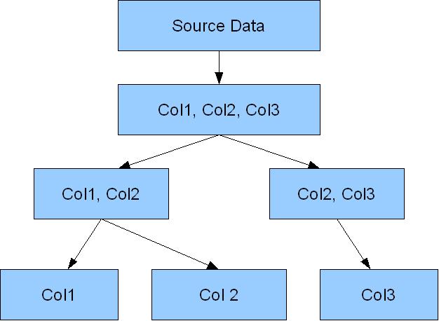
A HOLAP query potentially contains enough information for the optimizer to tell that there are result sets generated that can then be leveraged to produce further result sets. For example if you are going to aggregate at 10,000,000 row table and generate a 1,000,000 row result set for the grouping (col1, col2) then if the 1,000 row groupings (col1) and (col2) are also required then it makes sense to use the (col1, col2) result set to do so. On the other hand if two result sets (col1, col2) and (col2, col3) are required then there might be an advantage in calculating (col1, col2, col3) as an intermediate step, but it would depend on the sophistication of the optimization and the determination of whether such an intermediate step was worthwhile. If no intermediate set is produced then the original set of rows would be scanned twice, and as long as we can keep our sorts in memory we ought to be able to detect this.

When thinking about the possibilities for aggregation it makes sense to think of a tree structure of potential intermediate result sets, such as the following


That one shows promise for optimization by leveraging the intermediate result sets. However the following one does not:


I'm going to construct a slightly different test data set for this experiment, involving the aggregation of 10,000,000 by three different columns each having around 1000 distinct values. We will try aggregations at a number of different levels and combinations of levels, such as: ((COL1)), ((COL1),(COL2)), ((COL1),(COL1,COL2)), ((col1),(col2),(col3),(col1,col2,col3)), etc. with the intent of exposing us to almost a full range of potential optimizations.

The methodology for these tests is to execute each query four times, flushing the buffer cache before each one. The average statistics of the last three executions will be taken (with the intent that the recursive calls due to the hard parse of the first execution are thus excluded). Workarea size policy will be set to manual and sufficient sort area allocated to eliminate disk sorts. The host machine and database will be as quiescent as possible, which is not difficult to achieve in this environment.


.... And with that I'm going to break off this entry to let you absorb these ideas, comment back if you wish, and give me time to complete the tests.

ORA-12034: materialized view log younger than last refresh

Dabblers in the art of the materialisation of views may be used to seeing this error message, and it's often a portent of doom. Metalink Note 204127.1 tackles it head on with a list of possible causes, but is remiss in advising that a complete refresh is required.

And thank goodness for that. A multi-gigabyte materialized view based on a multi-multi-gigabyte master table is no joke to perform a complete refresh on, and anything we can do to avoid it is welcome.

As far as data warehousing is concerned we can trim the fat out of the Metalink note to shortlist our potential causes:
  • Previous refresh failed
  • Modifying the master table so that changes don't go to the materialized view log (truncate, alter partitions ... drop / truncate ... etc)
  • Master table reorganization
And here is another prime cause that the note doesn't identify:
  • Issuing an MV log purge.
All of these potential causes appear to be easily fixable through the simple mechanism of dropping and recreating the materialized view. But I'm not talking about dropping the data here. One of the requirements for this method to be successful is that the materialized view was created on a prebuilt table. If this is the case, and it is possible to find out if it is or not based on the BUILD_MODE column of USER_MVIEWS, then in the event of a refresh failure we can:
  1. Drop the materialized view.
  2. Do whatever is required (if anything) to bring the master table and the MV back into synchronization (delete data from master, or add data to MV).
  3. Recreate the MV, again using the ON PREBUILT TABLE clause obviously.
  4. Erm ...
  5. That's it.
Doubtless you script hounds will be wanting to see a test of this, huh?

create table m (col1 number);

create materialized view log on m
with rowid (col1)
including new values;

create table
m_mv_cstar
as
select count(*) c_star
from m;

create materialized view m_mv_cstar
on prebuilt table
refresh fast
on commit
as
select count(*) c_star
from m;

insert into m values (1);

commit;

That gets us a successfully fast refreshing materialized view. Now we break it.

drop materialized view log on m;

create materialized view log on m
with rowid (col1)
including new values;

insert into m values (1);

commit;


That ought to get you the ORA-12034 error, and this is the time to go and check whether any other materialized views has successfully refreshed and whether the change to the master table is still intact or whether that has been rolled back. In this case the change to m ought to have been rolled back.

So now we fix the problem of the ORA-12034 without a complete refresh of the materialized view.

drop materialized view m_mv;

create materialized view m_mv
on prebuilt table
refresh fast
on commit
as
select count(*) c_star
from m;

If by some chance you had mislaid the definition of your materialized view then use the following to retrieve it.

Set Long 100000 Pagesize 0

Select DBMS_Metadata.Get_DDL('MATERIALIZED_VIEW','M_MV_CSTAR') From Dual;

Note the underscore in the MATERIALIZED_VIEW there. Forget that and you'll receive a baffling:

1* Select DBMS_Metadata.Get_DDL('MATERIALIZED VIEW','M_MV_CSTAR') From Dual
SQL> /
ERROR:
ORA-31600: invalid input value MATERIALIZED VIEW for parameter OBJECT_TYPE in
function GET_DDL
ORA-06512: at "SYS.DBMS_METADATA", line 2576
ORA-06512: at "SYS.DBMS_METADATA", line 2627
ORA-06512: at "SYS.DBMS_METADATA", line 4220
ORA-06512: at line 1

So have we successfully recovered from the error?

insert into m values (1);

commit;

select * from m;

select * from m_mv_cstar;

Hopefully that demonstrates that we have.

So, is there a downside to this? Well if you have never run a complete refresh on your materialized view, or created it with a "build immediate" clause, then you will not get the comfort of a STALENESS of "FRESH" and will instead be stuck with the disturbing "UNKNOWN". Relax -- it's just that although you know that the materialized view is fresh, Oracle does not trust you. But then there are so many events that can break the "FRESH" staleness of your materialized view that you should treat FRESH MV's as a rare treat and not get used to them.

Yahoo Instant Messenger Out, Trillian In

Working remotely from my client as I do, I make a lot of use of instant messaging. I made the serious error of upgrading to the latest version and have watched in amusement as it's memory usage often goes northwards of hundreds of megabytes. The record was 1.2Gb ... nice!

Even when freshly started it squats there hogging 15Mb, and usually hovers between 30Mb and 50Mb, which is inexcusable for software that basically lets me type stuff to other people.

So Yahoo Instant Messenger is officially Bad Software, and I've replaced it with Trillian Basic 3.1 ... I'll be watching it very closely, but so far it hasn't done anything unpleasant and uses a fraction of the memory.

Wednesday, December 07, 2005

Brrrr ...

A little chilly this morning ... -2F/-19C

Oh, and guess who forgot to put the car in the garage last night?


Update: Guess who wisely decided to not put the car in the garage for fear of the garage door freezing immovably to the ground? That's right, me. I'm a genius.

Peterson AFB was on a two hour delay this morning, and the school district upgraded their two hour delay to a complete closure so I may be getting the company of a stir-crazy six year old boy. That'll be ... uh ... great.

On a positive note though, when it's this cold you don't find your vehicle encased in a solid sheet of ice in the morning. The snow just brushes straight off, sometimes into the top of an artfully placed boot.

It looks like it'll be hanging around a while as it's not due to get above freezing for a couple of days. We usually rely on sun + altitude + gravel to get the roads cleared, and it's pretty successful if you ignore the broken windshields and scratched paint. After our recent few days of cold our local roads are a sheet of inch-thick ice though, so that old advice that most accidents happen within five minutes of home is very true -- often five minutes can be only a hundred yards or so.

Tuesday, December 06, 2005

The Mysterious Benefit Of Completely Redundant Materialized Views

A Scenario


You've just started working on a new data warehouse project, and you're familiarizing yourself with the database schema. You are looking at a simple table that stores transactional information and which is defined as follows:

create table master
(
transaction_cd number not null,
location_cd number not null,
tx_timestamp date not null,
product_cd number not null,
tx_qty number not null,
tx_cst number not null
)
/
alter table master
add constraint xpkmaster primary key (transaction_cd)
/

Plus various foreign keys, indexes and other stuff of course.

Built upon this table are a number of materialized views, one of which has the following definition:

create materialized view
master_mv1
...
Enable Query Rewrite
As
Select
transaction_cd,
location_cd,
product_cd,
tx_timestamp,
sum(tx_qty) s_tx_qty,
sum(tx_cst) s_tx_cst,
count(*) c_star
from
master
group by
transaction_cd,
location_cd,
product_cd,
tx_timestamp
/

If you've spotted that all of the attribute columns of the master table are included in the materialized view, and one of those attributes is defined as the primary key of the master table, then you will correctly conclude the following: the materialized view is completely redundant. It stores exactly the same data as the master table.

So, simple question. Why go to the trouble of creating such an abominable waste of resources?

Answer below ...


Answer 1

It's because of a combination of problems.

Firstly, there are front-end tools that will not optimize their SQL to take account of situations where an aggregation of a metric is not required. A metric called "Transaction Qty" will commonly be defined as SUM(MASTER.TX_QTY) and will always be included in queries in the following way:

select
transaction_cd,
sum(tx_qty)
from
master
where
tx_timestamp between to_date('01-jan-2005')
and to_date('02-jan-2005') and
product_cd = 3
group by
transaction_cd
/

The front end tool will not recognise that when the primary key of the MASTER fact table is also selected then it is sufficient (and more efficient) to:

select
transaction_cd,
tx_qty
from
master
where
tx_timestamp between to_date('01-jan-2005')
and to_date('02-jan-2005') and
product_cd = 3
/

Now theoretically there is an opportunity for the Oracle optimizer to step in here and rescue us, but unfortunately it does not.

Here's a full demonstration script:

drop table master;
drop materialized view master_mv1;

create table master
(
transaction_cd not null,
location_cd not null,
tx_timestamp not null,
product_cd not null,
tx_qty not null,
tx_cst not null
)
pctfree 0
nologging
as
select
rownum,
trunc(dbms_random.value(1,10)),
to_date('01-jan-2005','DD-Mon-YYYY')
+ dbms_random.value(0,30),
trunc(dbms_random.value(1,10000)),
trunc(dbms_random.value(1,10)),
trunc(dbms_random.value(1,100),2)
from
dual
connect by
1=1 and
level < ownname =""> user,
tabname => 'master',
granularity => 'ALL');
end;
/

create materialized view master_mv1
nologging
Using No Index
Never Refresh
Enable Query Rewrite
As
Select
transaction_cd,
location_cd,
product_cd,
tx_timestamp,
sum(tx_qty) s_tx_qty,
sum(tx_cst) s_tx_cst
from
master
group by
transaction_cd,
location_cd,
product_cd,
tx_timestamp
/

begin
dbms_stats.gather_table_stats(
ownname => user,
tabname => 'master_mv1',
granularity => 'ALL');
end;
/

We can now compare the original and the rewritten queries and their execution plans:

explain plan for
select /*+ norewrite */
transaction_cd,
sum(tx_qty)
from master
where product_cd = 3
group by transaction_cd;

select * from table(dbms_xplan.display());
-----------------------------------------------------------------------------
| Id | Operation | Name | Rows | Bytes | Cost (%CPU)| Time |
-----------------------------------------------------------------------------
| 0 | SELECT STATEMENT | | 102 | 1224 | 792 (3)| 00:00:10 |
| 1 | SORT GROUP BY | | 102 | 1224 | 792 (3)| 00:00:10 |
|* 2 | TABLE ACCESS FULL| MASTER | 102 | 1224 | 791 (3)| 00:00:10 |
-----------------------------------------------------------------------------
explain plan for
select transaction_cd,
sum(tx_qty)
from master
where product_cd = 3
group by transaction_cd;
select * from table(dbms_xplan.display());
-------------------------------------------------------------------------------------------
| Id | Operation | Name | Rows | Bytes | Cost (%CPU)| Time |
-------------------------------------------------------------------------------------------
| 0 | SELECT STATEMENT | | 101 | 1212 | 874 (3)| 00:00:11 |
|* 1 | MAT_VIEW REWRITE ACCESS FULL| MASTER_MV1 | 101 | 1212 | 874 (3)| 00:00:11 |
-------------------------------------------------------------------------------------------

explain plan for
select transaction_cd,
sum(tx_qty)
from master
where location_cd = 3
group by transaction_cd;

select * from table(dbms_xplan.display());
-------------------------------------------------------------------------------------------
| Id | Operation | Name | Rows | Bytes | Cost (%CPU)| Time |
-------------------------------------------------------------------------------------------
| 0 | SELECT STATEMENT | | 111K| 1193K| 873 (3)| 00:00:11 |
|* 1 | MAT_VIEW REWRITE ACCESS FULL| MASTER_MV1 | 111K| 1193K| 873 (3)| 00:00:11 |
-------------------------------------------------------------------------------------------

Notice also that if we place a tempting index on the transaction_cd column of master_mv1 then we can get further benefits:

alter table master_mv1 add constraint xpk_master_mv1 primary key (transaction_cd)
/

explain plan for
select /*+ norewrite */
transaction_cd,
sum(tx_qty)
from master
where transaction_cd in (1,2,123456)
group by transaction_cd;

select * from table(dbms_xplan.display());
--------------------------------------------------------------------------------------------
| Id | Operation | Name | Rows | Bytes | Cost (%CPU)| Time |
--------------------------------------------------------------------------------------------
| 0 | SELECT STATEMENT | | 3 | 24 | 4 (0)| 00:00:01 |
| 1 | SORT GROUP BY NOSORT | | 3 | 24 | 4 (0)| 00:00:01 |
| 2 | INLIST ITERATOR | | | | | |
| 3 | TABLE ACCESS BY INDEX ROWID| MASTER | 3 | 24 | 4 (0)| 00:00:01 |
|* 4 | INDEX RANGE SCAN | XPK_MASTER | 3 | | 3 (0)| 00:00:01 |
--------------------------------------------------------------------------------------------

explain plan for
select transaction_cd,
sum(tx_qty)
from master
where transaction_cd in (1,2,123456)
group by transaction_cd;

select * from table(dbms_xplan.display());
---------------------------------------------------------------------------------------------------------
| Id | Operation | Name | Rows | Bytes | Cost (%CPU)| Time |
----------------------------------------------------------------------------------------------------------
| 0 | SELECT STATEMENT | | 3 | 24 | 4 (0)| 00:00:01 |
| 1 | INLIST ITERATOR | | | | | |
| 2 | MAT_VIEW REWRITE ACCESS BY INDEX ROWID| MASTER_MV1 | 3 | 24 | 4 (0)| 00:00:01 |
|* 3 | INDEX RANGE SCAN | XPK_MASTER_MV1 | 3 | | 3 (0)| 00:00:01 |
----------------------------------------------------------------------------------------------------------

Again, the sort group by phase is eliminated.

Answer 2:


Different groups of users may have different reporting priorities. Store managers will be applying filters such as "location_cd = 5", while product managers will be applying "product_cd = 123". Both of them would benefit from the physical clustering of similar values for the columns they usually apply filters to, through partitioning (and hence partition pruning) or through an insert of rows sorted by their favourite column, or maybe though clustering.

My bet would be on the master and the MV tables having different partitioning keys.

Now that's not the only way to "skin this cat" -- of course you might go down the path of composite partitioning. However that will give you a limited number of columns on which partition pruning is possible. For example with a multicolumn-range/list composite partitioning scheme on (A,B,C)/(D) you can get partition pruning for queries on the following combinations of predicated columns:

  • A

  • AB

  • ABC

  • ABCD

  • AD

  • ABD

The following combinations do not benefit from partition pruning:

  • B

  • C

  • BD

  • CD

  • BCD

It's actually possible though to benefit from partition pruning in those latter cases if a logically redundant predicate is placed on other columns ... for example if A had only distinct values of 'X','Y', and 'Z' then by including a predicate of:

A In ('X','Y','Z')

...then it is possible to extend the range of partition pruning ... erm ... well maybe I'll write another blog entry on that, but as you can see it's a little bit tricky and still requires some upfront planning.

So does the query rewrite costing take account of differences in partitioning pruning between a master table and it's materialized views?

drop table master;
drop materialized view master_mv1;

create table master
(
transaction_cd not null,
location_cd not null,
tx_timestamp not null,
product_cd not null,
tx_qty not null,
tx_cst not null
)
partition by list (location_cd)
(
partition p01 values (1),
partition p02 values (2),
partition p03 values (3),
partition p04 values (4),
partition p05 values (5),
partition p06 values (6),
partition p07 values (7),
partition p08 values (8),
partition p09 values (9),
partition p10 values (10)
)
pctfree 0
nologging
as
select
rownum,
trunc(dbms_random.value(1,10)),
to_date('01-jan-2005','DD-Mon-YYYY')
+ dbms_random.value(0,30),
trunc(dbms_random.value(1,10000)),
trunc(dbms_random.value(1,10)),
trunc(dbms_random.value(1,100),2)
from
dual
connect by
1=1 and
level < ownname =""> user,
tabname => 'master',
granularity => 'ALL');
end;
/

create materialized view master_mv1
partition by hash (product_cd)
partitions 256
compress nologging
Using No Index
Never Refresh
Enable Query Rewrite
As
Select
transaction_cd,
location_cd,
product_cd,
tx_timestamp,
sum(tx_qty) s_tx_qty,
sum(tx_cst) s_tx_cst
from
master
group by
transaction_cd,
location_cd,
product_cd,
tx_timestamp
/

begin
dbms_stats.gather_table_stats(
ownname => user,
tabname => 'master_mv1',
granularity => 'ALL');
end;
/

explain plan for
select transaction_cd,
sum(tx_qty)
from master
where product_cd = 3
group by transaction_cd;

select * from table(dbms_xplan.display());

explain plan for
select transaction_cd,
sum(tx_qty)
from master
where location_cd = 3
group by transaction_cd;

select * from table(dbms_xplan.display());

Here are the execution plans:

-------------------------------------------------------------------------------------------------------------
| Id | Operation | Name | Rows | Bytes | Cost (%CPU)| Time | Pstart| Pstop |
-------------------------------------------------------------------------------------------------------------
| 0 | SELECT STATEMENT | | 9 | 108 | 4 (25)| 00:00:01 | | |
| 1 | SORT GROUP BY | | 9 | 108 | 4 (25)| 00:00:01 | | |
| 2 | PARTITION HASH SINGLE | | 9 | 108 | 3 (0)| 00:00:01 | 36 | 36 |
|* 3 | MAT_VIEW REWRITE ACCESS FULL| MASTER_MV1 | 9 | 108 | 3 (0)| 00:00:01 | 36 | 36 |
-------------------------------------------------------------------------------------------------------------

---------------------------------------------------------------------------------------------------------
| Id | Operation | Name | Rows | Bytes |TempSpc| Cost (%CPU)| Time | Pstart| Pstop |
---------------------------------------------------------------------------------------------------------
| 0 | SELECT STATEMENT | | 11040 | 118K| | 63 (4)| 00:00:01 | | |
| 1 | SORT GROUP BY | | 11040 | 118K| 536K| 63 (4)| 00:00:01 | | |
| 2 | PARTITION LIST SINGLE| | 11040 | 118K| | 11 (0)| 00:00:01 | 3 | 3 |
| 3 | TABLE ACCESS FULL | MASTER | 11040 | 118K| | 11 (0)| 00:00:01 | 3 | 3 |
---------------------------------------------------------------------------------------------------------

We see here that the query is rewritten to take advantage of the different partitioning scheme of the materialized view. This simple case would have been a good candidate for a composite partitioning scheme of course.

The Cost Of Maintaining Redundant Materialized Views

So what is the cost to the system of providing this materialized view? Well if we're smart about how we maintain it then there is very little cost indeed. After all, we know that we don't have to aggregate the master data in order to populate the materialized view's table so I don't see why we would choose to do so.

In this previous blog I showed how there can be benefits to maintaining a materialized view manually, rather than through the internal refresh procedure. This redundant MV is an excellent example of a situation that benefits from such an approach, because the MV data is exactly the same as the master data. So instead of inserting the master table data and then refreshing the MV we can insert into both tables at the same time. As I noted before, the MV data can be maintained manually through either the partition exchange mechanism or by dropping the MV (if it is built on a predefined table) and directly inserting into it. In the latter case we could even use the multitable insert syntax that Oracle so thoughtfully provides to insert into both the master and the MV tables simultaneously, giving us the benefit of a single transaction.

Summary

So there we have it. Materialized views that are redundant in terms of data but which can provide interesting benefits in the report query phase.

Would I do such a thing myself? Maybe, maybe not. I don't believe that there ought to be qualms about the extra storage requirement because by the time you have used up half the capacity of todays hard drives you have already run out of bandwidth. I haven't worked in an environment where I have felt comfortable in implementing such a scheme, but I could see that I might. I can imagine a related situation where I would create a materialized view on a subset of the master table's columns in order to provide a skinny table (possibly with different partitioning scheme), in order to get the benefits of reduced i/o for scans of large number of rows and/or to leverage the optimizer's abandonment of the SORT GROUP BY phase when reporting on a primary key column.

Regardless of the practicality, I think that it serves as a nice demonstration of the power of query rewrite.

Monday, December 05, 2005

Dimensions Without Dimension Tables

Mike Ault has blogged on the subject here.

Thursday, December 01, 2005

Oracle Documentation Slow?

Is it just me or is the Oracle documentation site very slow right now? I keep getting timeouts on searching.

I feel like someone is stepping on my oxygen pipe when that happens.

Antivirus and Firewall Software Change

Norton is out, and AVS is in.

Norton has been killing my internet connection for a little while apparantly, but I only just found out that it was responsible when I noticed ccproxy.exe consuming 1.5Gb of memory and growing ... it's the kind of thing you tend to notice on a machine with 1.5Gb of physical memory plus Oracle EE 10gR1 running on it. I had to keep restarting the Symantec Netwrok Proxy service to restore the connection. "Bye-bye!"

So it turns out that not only does AVS have all the required credentials but it's user interface is also not nearly as funky as Norton's. It appears to do all the same stuff, plus it registers itself with Windows XP Security Center (which Norton never managed to do). The firewall part does everything I need as well.

Oh, and it's a darned sight cheaper as well -- the anti-virus part is free for home users, and AVG + Firewall Edition is a snip at $48.95 for a two year license.

Here you go: http://www.grisoft.com

(Their website is also much easier to use than Symantec's as well)